Neo All - example 2 - Cross-Correlograms¶

This example shows how to compute and plot cross-correlograms of spiketrains from different units.

First import neoStructures

from neoStructures import *
import matplotlib.pyplot as plt
from os.path import isdir, join

Import the data and create the NeoAll instance

data_dir = join('pySpikeAnalysis', 'sample_data') if isdir('pySpikeAnalysis') else join('..', '..', 'pySpikeAnalysis', 'sample_data')
spykingcircus_dir = r'SpykingCircus_results'
probe_filename = r'000_AA.prb'
results_filename = r'spykingcircusres'

neoAll = NeoAll(join(data_dir, spykingcircus_dir), results_filename, join(data_dir, probe_filename), save_fig=0)

See information about NeoAll

print(neoAll)

Out:

NeoAll Instance with 54 units. 1 Neo segment per unit. Each segment contains 1 Neo spiketrain
10 channel indexes

Use neoStructures.NeoAll.plot_crosscorrelogram() to plot cross-correlogram between 2 units. The spiketrains are first converted into binned spiketrains before the computation of the cross-correlogram. The package Elephant is used for the binning as well as for computing the cross-correlogram. Let’s compute the cross-correlogram between the first 2 units :

neoAll.plot_crosscorrelogram(0, 1)

We can see from these cross-correlogram that the two units often fire together Bin duration is set by default to 1ms but can be modified. The max_lag_time parameter sets the time limits of the cross-correlogram, its default value is set to 80 ms It can be changed to zoom on the peak near the origin :

neoAll.plot_crosscorrelogram(0, 1, bin_time=1*ms, max_lag_time=25*ms)

Some statistics can be computed, be setting the do_stat parameter to 1 : n_surrogates spike-trains are created in which a jitter is added to the time of the spikes. The jitter is computed from a normal distribution whose standard deviation is fixed by the normal_dist_sd parameter. The 99% confidence interval computed from the jittered spiketrains is shown on top of the cross-correlogram.

neoAll.plot_crosscorrelogram(0, 1, do_stat=True, n_surrogates=20, normal_dist_sd=25*ms)

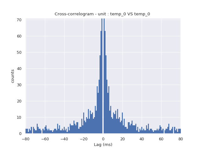
If unit_pos_a and unit_pos_b parameters are equals, the autocorrelogram is computed.

neoAll.plot_crosscorrelogram(0, 0)

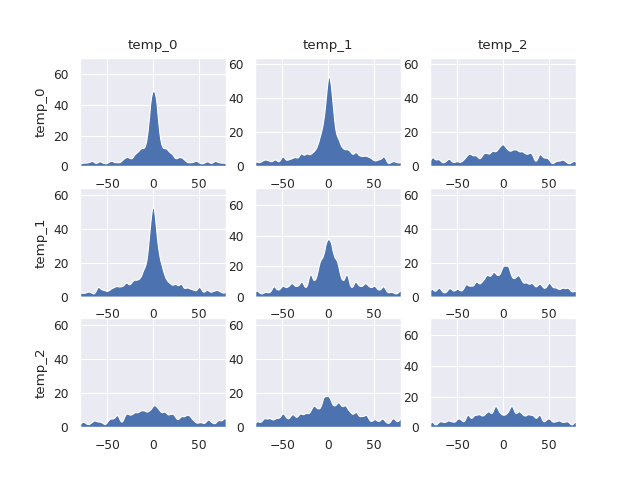
Multiples cross-correlogram can be plot at the same time in multiple figures :

neoAll.plot_crosscorrelogram(0, [0, 1, 2])

Or in the same figure :

neoAll.plot_crosscorrelogram([0, 1, 2], [0, 1, 2], merge_plots=1)

If same_yscale is True, the cross-correlograms are smoothed and the same y-scale is used.

neoAll.plot_crosscorrelogram([0, 1, 2], [0, 1, 2], merge_plots=1, same_yscale=1, fill_under_plot=1)

Total running time of the script: ( 0 minutes 6.766 seconds)

Gallery generated by Sphinx-Gallery